Part I
In Part I we made a connection to a SQLite DB.
What are we tackling in Part II?
- We’ll do more advanced
dplyr📦 workflows. - We’ll collect the data from the query.
The project on GitHub, has the example SQLite database, the slides, and some code files.
Connect, and remind ourselves what we’re working with
Make a connection
As always, our first step is to connect to the database.
library(DBI) # main DB interface
library(dplyr)
library(dbplyr) # dplyr back-end for DBs

con <- dbConnect(drv = RSQLite::SQLite(), # give me a SQLite connection
        dbname = "data/great_brit_bakeoff.db") # To what? The DB named great_brit_bakeoff.db

dbListTables(con) # List me the tables at the connection
 [1] "baker_results"     "bakers"            "bakes"
 [4] "challenge_results" "challenges"        "episode_results"
 [7] "episodes"          "ratings"           "ratings_seasons"
[10] "results"           "seasons"           "series"
Let’s get familiar with our data
In the dataset we have:
- results which tells us how each baker did in the episode -
IN,OUT,WINNERetc. - baker_results which tells us a bit more about the baker’s performance over the entire series - how many times did they win
STAR BAKER, how many times they placed in the top 3 etc.
Let’s get an idea of what is in each table.
results
tbl(con, "results") %>% # Reach into my connection, and "talk" to results table
  head(10) %>%          # get me a subset of the data
  # sometimes if there are many columns, some columns are hidden,
  # this option prints all columns for us
  print(width = Inf)
# Source:   lazy query [?? x 4]
# Database: sqlite 3.36.0 [C:\Users\Vebashini\OneDrive -
#   Rain\Documents\Main-Documents\Personal\Blog_Vebash\_posts\2020-12-20-using-the-tidyverse-with-dbs-partii\data\great_brit_bakeoff.db]
   series episode baker   result
    <int>   <int> <chr>   <chr>
 1      1       1 Annetha IN
 2      1       2 Annetha OUT
 3      1       3 Annetha <NA>
 4      1       4 Annetha <NA>
 5      1       5 Annetha <NA>
 6      1       6 Annetha <NA>
 7      1       1 David   IN
 8      1       2 David   IN
 9      1       3 David   IN
10 1 4 David OUT # Source: lazy query [?? x 2]
# Database: sqlite 3.36.0 [C:\Users\Vebashini\OneDrive -
# Rain\Documents\Main-Documents\Personal\Blog_Vebash\_posts\2020-12-20-using-the-tidyverse-with-dbs-partii\data\great_brit_bakeoff.db]
# Ordered by: desc(n)
result n
<chr> <int>
1 IN 452
2 <NA> 376
3 OUT 79
4 STAR BAKER 70
5 RUNNER-UP 18
6 WINNER 9
7 [a] 1
8 WD 1baker_results
tbl(con, "baker_results") %>% # Reach in and "talk" to baker_results
  head() %>%                  # get a glimpse of data
  collect() %>%               # bring that glimpsed data into R
  DT::datatable(options = list(scrollX = TRUE)) # force DT horizontal scrollbar
Notice the use of the collect() function in the code above. I wanted us to be able to get a full glimpse of the data in a nice table, and hence I brought the first few rows of data into R by using the collect() function. This allowed me to then use datatable to display the results a bit better, than the print(width = Inf) alternative.
What are we interested in?
Let’s say we want to see how the WINNER and RUNNER-UP(s) did in the series they appeared in.
To do that we need to get all the baker_results for the WINNER and RUNNER-UP.
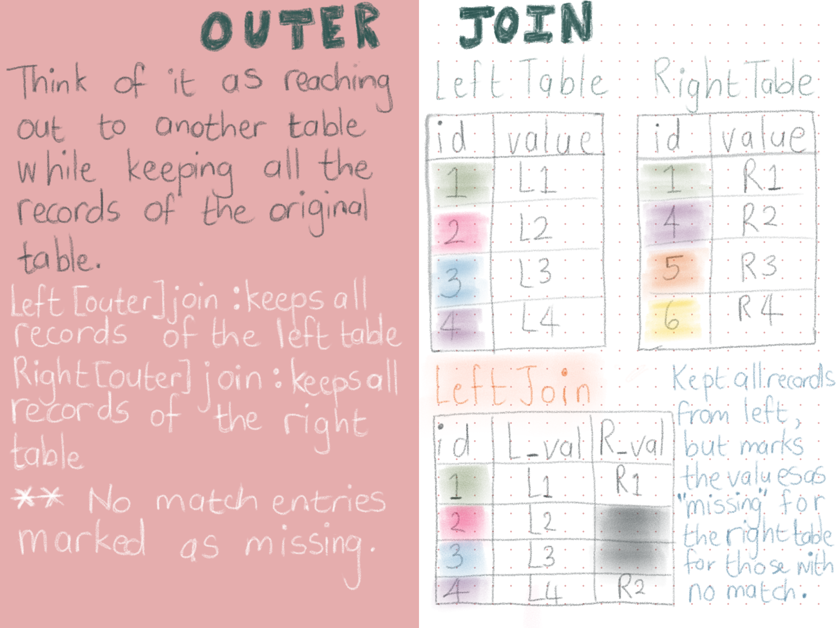
Joining data
When doing joins we want to find the common columns across the two tables that we can join on.
- In results we have
seriesandbaker. - In baker_results we have
seriesandbaker. - ❓ 🤔 Why didn’t I also choose the
episodecolumn of results as a join column?
✅ Yes, that column is not inbaker_results, sincebaker_resultscontains data about how the baker did overall in the series they appeared, that is, one row per baker.
Theresultsdata however, contains info per baker, per episode, for the series they appeared in - i.e. if they flopped (wereOUT😉), in the second episode of a series that contained 10 episodes, their name would appear 10 times in theresultstable, but their “result” value will beNAfrom episode 3 onwards.
Remember the tbl(con, "tbl_name") always
I’d like to bring to your attention the use of tbl(con, "table_1") and tbl(con, "table_2") in the join function.
We must always keep this in mind, because baker_results and results don’t exist in R yet. We’re talking to those tables in our relational database management system (RDBMS), so we always have to do so through our connection.
set.seed(42)
tbl(con, "baker_results") %>% # use connection to "talk" to baker_results
  inner_join(tbl(con, "results"), # use connection to "talk" to results and join both tables
        by = c('baker' = 'baker',
               'series' = 'series')) %>% # join criteria
  collect() %>% # get it into R
  sample_n(size = 3) %>% # take a random sample
  print(width = Inf) # print all columns
# A tibble: 3 x 26
  series baker_full     baker     age occupation
   <dbl> <chr>          <chr>   <dbl> <chr>
1      6 Ian Cumming    Ian        41 Travel photographer
2      4 Frances Quinn  Frances    31 Children's Clothes Designer
3      2 Yasmin Limbert Yasmin     43 Childminder
  hometown                          baker_last baker_first star_baker
  <chr>                             <chr>      <chr>            <int>
1 Great Wilbraham, Cambridgeshire   Cumming    Ian                  3
2 Market Harborough, Leicestershire Quinn      Frances              1
3 West Kirby, The Wirral            Limbert    Yasmin               1
  technical_winner technical_top3 technical_bottom technical_highest
             <int>          <int>            <int>             <dbl>
1                1              6                4                 1
2                1              7                3                 1
3                0              2                4                 2
  technical_lowest technical_median series_winner series_runner_up
             <dbl>            <dbl>         <int>            <int>
1                8                3             0                1
2                8                3             1                0
3                6                5             0                0
  total_episodes_appeared first_date_appeared last_date_appeared
                    <dbl>               <dbl>              <dbl>
1                      10               16652              16715
2                      10               15937              16000
3                       6               15202              15237
  first_date_us last_date_us percent_episodes_appeared
          <dbl>        <dbl>                     <dbl>
1         16983        17025                       100
2         16432        16495                       100
3            NA           NA                        75
  percent_technical_top3 episode result
                   <dbl>   <int> <chr>
1                   60         5 IN
2                   70         5 IN
3                   33.3       5 IN
Notice that all columns of baker_results appear first and then we have the “extra” columns from results i.e. episode and result.
Common mistake
I included the above to show that each time we “talk” to a table we must do so through our connection, because I often make the mistake of not including the tbl(con, "name_of_tbl_i_am_joining") in the join function. I, more times than I care to admit 🤦♀️, incorrectly write:
  tbl(con, "table1") %>% # correct -> "talk" through connection
     left_join(table2,   # incorrect -> forgot to use the connection
          by = c("tbl1_name1" = "tbl2_name1"))
I would like to help you, not repeat my mistake 😕, so heads up AVOID THE FOLLOWING 🛑:
tbl(con, "baker_results") %>% # use connection to "talk" to baker_results
  inner_join(results,  # OOPS! I forgot the tbl(con, "results")
        by = c('baker' = 'baker',
               'series' = 'series'))
Error in tbl_vars_dispatch(x): object 'results' not foundCollect
Ok, let us now do our entire pipeline, and only bring the data into R when we’ve got what we’re looking for.
We need to:
- Join the tables
- Filter the data for
WINNERandRUNNER-UPin the result column. - Select only the columns we’re interested in.
(final_query <- tbl(con, "baker_results") %>% # use connection to "talk" to baker_results
  inner_join(tbl(con, "results"), # use connection to "talk" to results and join both tables
        by = c('baker' = 'baker',
               'series' = 'series')) %>% # join criteria
  filter(result %in% c("WINNER", "RUNNER-UP")) %>% # filter rows we're interested in
  select(series, baker:percent_technical_top3,
         result))
# Source:   lazy query [?? x 24]
# Database: sqlite 3.36.0 [C:\Users\Vebashini\OneDrive -
#   Rain\Documents\Main-Documents\Personal\Blog_Vebash\_posts\2020-12-20-using-the-tidyverse-with-dbs-partii\data\great_brit_bakeoff.db]
   series baker       age occupation  hometown  baker_last baker_first
    <dbl> <chr>     <dbl> <chr>       <chr>     <chr>      <chr>
 1      1 Edd          24 Debt colle~ Bradford  Kimber     Edward
 2      1 Miranda      37 Food buyer~ Midhurst~ Browne     Miranda
 3      1 Ruth         31 Retail man~ Poynton,~ Clemens    Ruth
 4      2 Holly        31 Advertisin~ Leicester Bell       Holly
 5      2 Joanne       41 Housewife   Ongar, E~ Wheatley   Joanne
 6      2 Mary-Anne    45 Housewife   Kiddermi~ Boermans   Mary-Anne
 7      3 Brendan      63 Recruitmen~ Sutton C~ Lynch      Brendan
 8      3 James        21 Medical st~ Hillswic~ Morton     James
 9      3 John         23 Law student Wigan     Whaite     John
10      4 Frances      31 Children's~ Market H~ Quinn      Frances
# ... with more rows, and 17 more variables: star_baker <int>,
#   technical_winner <int>, technical_top3 <int>,
#   technical_bottom <int>, technical_highest <dbl>,
#   technical_lowest <dbl>, technical_median <dbl>,
#   series_winner <int>, series_runner_up <int>,
#   total_episodes_appeared <dbl>, first_date_appeared <dbl>,
#   last_date_appeared <dbl>, first_date_us <dbl>, ...
The above code just sets up the query that will be executed should we run (Ctrl + Enter) final_query in R (hence the lazy query [?? x 24] in the output). No data is collected (i.e. present in your local R environment) as yet.
What does the query look like?
final_query %>%
  show_query()
<SQL>
SELECT `series`, `baker`, `age`, `occupation`, `hometown`, `baker_last`, `baker_first`, `star_baker`, `technical_winner`, `technical_top3`, `technical_bottom`, `technical_highest`, `technical_lowest`, `technical_median`, `series_winner`, `series_runner_up`, `total_episodes_appeared`, `first_date_appeared`, `last_date_appeared`, `first_date_us`, `last_date_us`, `percent_episodes_appeared`, `percent_technical_top3`, `result`
FROM (SELECT `LHS`.`series` AS `series`, `baker_full`, `LHS`.`baker` AS `baker`, `age`, `occupation`, `hometown`, `baker_last`, `baker_first`, `star_baker`, `technical_winner`, `technical_top3`, `technical_bottom`, `technical_highest`, `technical_lowest`, `technical_median`, `series_winner`, `series_runner_up`, `total_episodes_appeared`, `first_date_appeared`, `last_date_appeared`, `first_date_us`, `last_date_us`, `percent_episodes_appeared`, `percent_technical_top3`, `episode`, `result`
FROM `baker_results` AS `LHS`
INNER JOIN `results` AS `RHS`
ON (`LHS`.`baker` = `RHS`.`baker` AND `LHS`.`series` = `RHS`.`series`)
)
WHERE (`result` IN ('WINNER', 'RUNNER-UP'))
Bring it into R
Now finally, we are ready to bring our filtered and joined data into R by using collect().
(top_performers <- final_query %>%
  collect())
# A tibble: 24 x 24
   series baker       age occupation  hometown  baker_last baker_first
    <dbl> <chr>     <dbl> <chr>       <chr>     <chr>      <chr>
 1      1 Edd          24 Debt colle~ Bradford  Kimber     Edward
 2      1 Miranda      37 Food buyer~ Midhurst~ Browne     Miranda
 3      1 Ruth         31 Retail man~ Poynton,~ Clemens    Ruth
 4      2 Holly        31 Advertisin~ Leicester Bell       Holly
 5      2 Joanne       41 Housewife   Ongar, E~ Wheatley   Joanne
 6      2 Mary-Anne    45 Housewife   Kiddermi~ Boermans   Mary-Anne
 7      3 Brendan      63 Recruitmen~ Sutton C~ Lynch      Brendan
 8      3 James        21 Medical st~ Hillswic~ Morton     James
 9      3 John         23 Law student Wigan     Whaite     John
10      4 Frances      31 Children's~ Market H~ Quinn      Frances
# ... with 14 more rows, and 17 more variables: star_baker <int>,
#   technical_winner <int>, technical_top3 <int>,
#   technical_bottom <int>, technical_highest <dbl>,
#   technical_lowest <dbl>, technical_median <dbl>,
#   series_winner <int>, series_runner_up <int>,
#   total_episodes_appeared <dbl>, first_date_appeared <dbl>,
#   last_date_appeared <dbl>, first_date_us <dbl>, ...
How about that? Notice the A tibble: 24 x 24! R now, has the data in it’s local environment, and can definitively tell us it knows there are 24 observations (no more lazy query) 😄.
Visualise Data
Now that we have finalised what data we wanted from our RDBMS, executed our query, and collected the data into our R environment we can do further processing, create plots for reports etc.
I am interested in understanding how did the winner and runner-up(s) of series 6 do across the season in terms of technical challenges etc.?
library(tidyverse)

top_performers %>%
  # filter for season we're interested in
  filter(series == 6) %>%
  # format baker nicely so we see winner, then runner-up(s)
  mutate(baker_name = factor(str_glue("{result} - {baker}")),
         baker_name = fct_rev(baker_name)) %>%
  # let's convert all the tech info cols to be a metric name,
  # and put the value in the value column
  # (by default values_to = "value" in pivot_longer())
  pivot_longer(cols = c(star_baker:technical_median),
               names_to = "metric") %>%
  mutate(metric = fct_reorder(metric, value)) %>%
  ggplot(aes(x = value, y = metric)) +
  geom_col(fill = "#727d97") +
  facet_wrap(~ baker_name) +
  labs(title = str_glue("Metrics for Season ",
    "{top_performers %>%  filter(series == 6) %>%
    select(series) %>% distinct()}'s Winner and Runner-Up(s)"),
    y = "") +
  theme_light() +
  theme(panel.spacing = unit(1, "lines")) +
  theme(strip.background =element_rect(fill="#f4e4e7"))+
  theme(strip.text = element_text(colour = "#5196b4"))
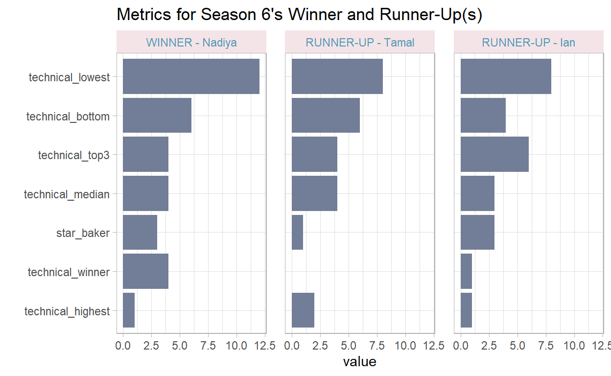
Given that Nadiya was a technical winner more times than the other contestants, and that her technical_lowest was better (higher number is better) it looks like she had a good run throughout the series, and was a deserved winner.
Done? Remember to disconnect!
Good housekeeping means always remembering to disconnect once you’re done.
dbDisconnect(con) # closes our DB connection
Still to come
- Setting up an external DB in PostgreSQL / MySQL.
- Connecting to said DB, and running SQL workloads on it.
Acknowledgements
The Great British Bake Offdata from Dr. Alison Hill.- Edgar Ruiz’s database work, and teachings.