No need to be a scared-y cat, “A lot of good tricks. I will show them to you. Your mother will not mind at all if I do.”

Photo by MIKHAIL VASILYEV on Unsplash
Terminology
To set the stage, let’s talk about the types of data. These are concepts more for beginners, so if you’re familiar with these please feel free to skip ahead.
We have two types of data:
- Numerical data, also known as
Quantitativedata. - Non-Numerical data, also known as
Qualitativedata (this is what we will be concentrating on in this post).
Numerical (Quantitative) data
Takes on number values:
Discrete: These are for example, count values: 0, 1, 2 - how many people took the survey, how many cats do you have in your home, how many children (aged below 18) are there in a household?
Continuous: These are numbers that can take on infinite values within some range of values - percentage of survey filled by respondents (e.g. 21.562%, 67.893%, 90.145%), heights of siberian cats (30.167 cm, 31.458 cm, 28.624 cm).
It makes sense to take the average of numerical data, and to do other arithmetic on numerical data, such as to add, subtract etc.
For example, it’s easy to say, in our sample the tallest siberian cat is 1.291 centimetres taller than the shortest siberian cat.
Non-Numerical (Qualitative) data
Also known as categorical data, since it can take on some number of distinct categories e.g. eye colour (brown, blue, green, grey etc.), favourite rock band, even names if you think about it, fall under categorical data, albeit many distinct categories may be present in such a
namevariable, and we therefore typically treat those kinds of non-numerical fields as pure character data.The categories are limited, and distinct - Siberian cat, Cornish Rex, Russian Blue - and may therefore be represented as numbers. In R each distinct category is referred to as a level.
- For example, you may have a survey question with the following categories:
Category Level Number Very Likely 1 Likely 2 Uncertain 3 Unlikely 4 Very Unlikely 5 There are 5 levels.
- Or, you may have a question asking a participant which of your favourite songs they enjoy the most, with the following categories:
Category Level Number Sweet Child O’ Mine 1 Smells Like Teen Spirit 2 Hotel California 3 Best of You 4 Numb 5 Unfamiliar with all of these 6 There are 6 levels.
The numbers (
Level Number) are basically placeholders for each category level, and is meant for us to work with it easier in a programming language. If I get the responses:
      Numb, Smells Like Teen Spirit, Sweet Child O' Mine, Smells Like Teen Spirit, Numb,
      Smells Like Teen Spirit, Sweet Child O' Mine, Numb, Smells Like Teen Spirit, Numb,
      Sweet Child O' Mine, Sweet Child O' Mine, Smells Like Teen Spirit

      I.e. 5, 2, 1, 2, 5, 2, 1, 5, 2, 5, 1, 1, 2
I can’t say Numb is 4x better, or 4x worse than Sweet Child O’ Mine (in other words, it makes no sense to take Level Number of Numb [5], and subtract Level Number of Sweet Child ’O Mine [1]).
Neither can I say that Hotel California is the average category chosen (notice it was not chosen once) but if I take the average of the numerical placeholders for the responses received, I would get 2.62 which is 3 if I round up. In other words, we can’t understand what the “average” song is.
So we have seen that it does not make sense to do arithmetic on these variables. The distance between the categories is not something that can be measured.
We can count each category, and understand that Smells Like Teen Spirit was the most popular among respondents.
Categorical data may be:
- Unordered, often refered to merely as Categorical data, or also known as
Nominaldata. For example, if your question is “What's your favourite Altoids flavour?” with the following options, while you may rank Cinnamon above Wintergreen there is no order to these categories! 😁.
Fave Flavour Level Number Peppermint 1 Wintergreen 2 Cinnamon 3 Spearmint 4 Liqourice 5 None of these 6 - Ordered, and hence called
Ordinaldata. Here’s an example using age categories - these are not numerical data, because theLevel Numberis merely a placeholder for the category, and we can’t do arithmetic on these. This is anOrdinalvariable however, since there is some order to the distinct categories shown inAge Range.
Age Range Level Number Younger than 21 1 21-30 2 31-45 3 46-55 4 Older than 55 5 - Unordered, often refered to merely as Categorical data, or also known as
{forcats} 📦
The forcats 📦 is meant to handle factors which is R’s data type for categorical data. forcats is for categorical data, and is an anagram for factors 🆒.
The functions in the package start with fct_.
There is non-numeric data where it is useful to work with the data as factors (age-ranges, occupation, etc.), but we must also keep in mind that some non-numeric data should be kept as character data.
We’re going to work with non-numeric data that may be treated as factors in this post, and learn how to use the forcats 📦 to make that task easier for us.
Data
We’re going to use the data from the awesome TidyTuesday Project ✨:
library(tidyverse)
brewing_materials <-
   read_csv(
    # hacky solution to show readers the full path of file
    # str_glue just pastes the various strings next to each other
    str_glue('https://raw.githubusercontent.com/rfordatascience/',
            'tidytuesday/master/data/2020/2020-03-31/',
            'brewing_materials.csv'))
beer_taxed <-
    read_csv(
     str_glue('https://raw.githubusercontent.com/rfordatascience/',
              'tidytuesday/master/data/2020/2020-03-31/',
              'beer_taxed.csv'))

brewer_size <-
    read_csv(
     str_glue('https://raw.githubusercontent.com/rfordatascience/',
     'tidytuesday/master/data/2020/2020-03-31/',
     'brewer_size.csv'))

beer_states <-
    read_csv(
     str_glue('https://raw.githubusercontent.com/rfordatascience/',
     'tidytuesday/master/data/2020/2020-03-31/',
     'beer_states.csv'))

beer_awards <-
    read_csv(
     str_glue('https://raw.githubusercontent.com/rfordatascience/',
     'tidytuesday/master/data/2020/2020-10-20/',
     'beer_awards.csv'))
Let’s have a look at the data - here we’re showing a sample from each table.
Show code
Show code
Show code
Show code
Show code
Convert variable to factor
To convert a variable to a factor we use factor() / as.factor() or forcats::as_factor(). These functions converts each distinct category to some number placeholder in the background.
Let’s get a better feel for the non-numeric data in the datasets we will be considering here.
brewing_materials
Let’s have a look at the material_type and type fields in the brewing_materials dataset.
brewing_materials %>%
  count(material_type)
# A tibble: 5 x 2
  material_type                n
  <chr>                    <int>
1 Grain Products             600
2 Non-Grain Products         480
3 Total Grain products       120
4 Total Non-Grain products   120
5 Total Used                 120
brewing_materials %>%
count(type)
# A tibble: 12 x 2
   type                           n
   <chr>                      <int>
 1 Barley and barley products   120
 2 Corn and corn products       120
 3 Hops (dry)                   120
 4 Hops (used as extracts)      120
 5 Malt and malt products       120
 6 Other                        120
 7 Rice and rice products       120
 8 Sugar and syrups             120
 9 Total Grain products         120
10 Total Non-Grain products     120
11 Total Used                   120
12 Wheat and wheat products     120
brewing_materials %>%
filter(stringr::str_to_lower(material_type) %in%
c('grain products',
'non-grain products')) %>%
count(material_type, type)
# A tibble: 9 x 3
  material_type      type                           n
  <chr>              <chr>                      <int>
1 Grain Products     Barley and barley products   120
2 Grain Products     Corn and corn products       120
3 Grain Products     Malt and malt products       120
4 Grain Products     Rice and rice products       120
5 Grain Products     Wheat and wheat products     120
6 Non-Grain Products Hops (dry)                   120
7 Non-Grain Products Hops (used as extracts)      120
8 Non-Grain Products Other                        120
9 Non-Grain Products Sugar and syrups             120
factor() / as.factor()
These are conversion functions to convert a variable to a factor in Base R.
To convert a variable to a factor we may use:
df <- df %>% mutate(var = factor(var))df <- df %>% mutate(var = as.factor(var))
To figure out what number placeholder a category was given behind the scenes, use
levels().The default order of
factor()is sorted. According to the help page: “The levels of a factor are by default sorted, but the sort order may well depend on the locale at the time of creation, and should not be assumed to be ASCII.”brewing_materials %>% mutate(material_type = factor(material_type)) %>% # use dplyr::pull which acts like $ to get the variable pull(material_type) %>% # let us get the number placeholder attached to each category levels()[1] "Grain Products" "Non-Grain Products" [3] "Total Grain products" "Total Non-Grain products" [5] "Total Used"brewing_materials %>% mutate(material_type = as.factor(material_type)) %>% # can also use count() to count how many in each level count(material_type)# A tibble: 5 x 2 material_type n <fct> <int> 1 Grain Products 600 2 Non-Grain Products 480 3 Total Grain products 120 4 Total Non-Grain products 120 5 Total Used 120Notice that the base R functions
factor()/as.factor()createdlevelsin the alphabetical sorted order (my locale is ASCII). The output of the first part of the code block shows that"Grain Products"was coded as 1, while"Total Non-Grain products"was coded as 4, and"Total Used"was coded as the last level which was 5.What if I wanted to specify the levels myself? I could specify the levels in an argument as shown:
levels = c("Level1", ..., "LevelN").brewing_materials %>% mutate(material_type = factor(material_type, # I want to make a factor but I want the order to be # as follows: levels = c("Grain Products", "Total Grain products", "Non-Grain Products", "Total Non-Grain products", "Total Used"))) %>% pull(material_type) %>% levels()[1] "Grain Products" "Total Grain products" [3] "Non-Grain Products" "Total Non-Grain products" [5] "Total Used"My level specification is used to create the levels, so the numeric encoding follows my specification this time.
"Total Grain products"is coded as level 2 this time (it was level 3 in the default creation where nolevelsargument was specified).What if I wanted to include levels that may exist in future datasets, but don’t as yet in the dataset we have? This is similar to the
monthsexample in R for Data Science. Let’s try it with adding a Not Applicable level, which is not in our dataset’smaterial_typevariable.brewing_materials %>% mutate(material_type = factor(material_type, levels = c("Grain Products", "Total Grain products", "Non-Grain Products", "Total Non-Grain products", "Total Used", "Not Applicable"))) %>% pull(material_type) %>% levels()[1] "Grain Products" "Total Grain products" [3] "Non-Grain Products" "Total Non-Grain products" [5] "Total Used" "Not Applicable"Has it been created?
brewing_materials %>%
   mutate(material_type = factor(material_type,
                           levels = c("Grain Products",
                                      "Total Grain products",
                                      "Non-Grain Products",
                                      "Total Non-Grain products",
                                      "Total Used",
                                      "Not Applicable"))) %>%
   # we can also count as before but notice that
   # one category that has no data is missing -
   # the artificial `Not Applicable` we added
   count(material_type)
# A tibble: 5 x 2 material_type n <fct> <int> 1 Grain Products 600 2 Total Grain products 120 3 Non-Grain Products 480 4 Total Non-Grain products 120 5 Total Used 120A simple
count()does not quite let us know, but if we add an argument.drop = FALSEwe get counts for all categories, even those with no observations (i.e. that category has a count of 0). By default thecount()function drops categories with 0 counts from the output. By adding.drop = FALSEwe’re asking for these to be included.brewing_materials %>% mutate(material_type = factor(material_type, levels = c("Grain Products", "Total Grain products", "Non-Grain Products", "Total Non-Grain products", "Total Used", "Not Applicable"))) %>% # we can get all categories by adding the .drop = FALSE count(material_type, .drop = FALSE)# A tibble: 6 x 2 material_type n <fct> <int> 1 Grain Products 600 2 Total Grain products 120 3 Non-Grain Products 480 4 Total Non-Grain products 120 5 Total Used 120 6 Not Applicable 0
forcats::as_factor()
as_factor() behaves differently to as.factor() in that it creates levels in the order in which they appear, hence we get the same factor levels across different locales.
Base R’s as.factor()
test_factor_var <-  c("012star", "DogsRule", "!this", "%abc",
            "Abc#", "abc$", "$bb", "AreYouKiddingCatsRule!")

test_factor_var %>%
  as.factor() %>%
  print(width = Inf)
[1] 012star                DogsRule
[3] !this                  %abc
[5] Abc#                   abc$
[7] $bb                    AreYouKiddingCatsRule!
Levels: !this $bb %abc 012star Abc# abc$ AreYouKiddingCatsRule! DogsRule
Note that the levels (seen in the output Levels: !this $bb ...) follow the [ASCII] sort on my machine, this may be completely different based on your locale.
Contrast with forcats::as_factor()
Now let’s consider as_factor().
# here is the raw variable again
test_factor_var
[1] "012star"                "DogsRule"
[3] "!this"                  "%abc"
[5] "Abc#"                   "abc$"
[7] "$bb"                    "AreYouKiddingCatsRule!"
# Now let's make it a factor, this time using
# as_factor()
test_factor_var %>%
as_factor() %>%
print(width = Inf)
[1] 012star                DogsRule
[3] !this                  %abc
[5] Abc#                   abc$
[7] $bb                    AreYouKiddingCatsRule!
Levels: 012star DogsRule !this %abc Abc# abc$ $bb AreYouKiddingCatsRule!
Note that as_factor() kept the order as it appears (Levels: 012star DogsRule ...), this will be the same for you, even if your locale is different.
Convert brewer data
Let’s perform the same conversion we did with Base R functions, but now using forcats::as_factor().
First let’s have a look at the default order that
as_factor()creates the variable in.brewing_materials %>% pull(material_type) %>% # what order are material_type observations in? head(12)[1] "Grain Products" "Grain Products" [3] "Grain Products" "Grain Products" [5] "Grain Products" "Total Grain products" [7] "Non-Grain Products" "Non-Grain Products" [9] "Non-Grain Products" "Non-Grain Products" [11] "Total Non-Grain products" "Total Used"brewing_materials %>% mutate(material_type = as_factor(material_type)) %>% pull(material_type) %>% levels()[1] "Grain Products" "Total Grain products" [3] "Non-Grain Products" "Total Non-Grain products" [5] "Total Used"Notice the levels are created in the order they appear in the
material_typefield -"Grain Products"appeared first hence is Level 1,"Total Grain products"appeared second hence occupies Level 2.
fct_inorder()
We can also explicitly use the fct_inorder() function to reorder the factor levels by first appearance. I add it here just so you’re aware of this option.
For example, the beer_awards$medal column would be made alphabetical in my locale if I use as.factor().
beer_awards %>%
  head(3)
# A tibble: 3 x 7
  medal  beer_name        brewery      city    state category     year
  <chr>  <chr>            <chr>        <chr>   <chr> <chr>       <dbl>
1 Gold   Volksbier Vienna Wibby Brewi~ Longmo~ CO    American A~  2020
2 Silver Oktoberfest      Founders Br~ Grand ~ MI    American A~  2020
3 Bronze Amber Lager Skipping Ro~ Staunt~ VA American A~ 2020[1] "Bronze" "Gold" "Silver"Notice the alphabetical ordering of levels (Bronze, Gold, Silver).
If I follow this with a fct_inorder() the ordering of levels is now using the order of appearance instead.
[1] "Gold" "Silver" "Bronze"In most cases we’d want this to be Bronze, Silver, Gold in order of increasing award type. We’ll see how to do that just now.
Manually order levels
fct_relevel()
Now we may specify the order ourselves (i.e. manually order the levels) by using
fct_relevel(). For example, as we talked about previously, we may want the award medals to be ordered Bronze, Silver, Gold in order of increasing award type, instead of order of appearance (or Base R’s alpha sorting in my locale).beer_awards %>% # I want to specify my factor levels myself mutate(medal = fct_relevel(medal, # we want a specific order, and # the order in which the categories # appear does not meet that specification "Bronze", "Silver", "Gold")) %>% pull(medal) %>% levels()[1] "Bronze" "Silver" "Gold"We can’t add a level that is not in the dataset, or we can, but we get a Warning), and the level is not added.
brewing_materials_forcats <- brewing_materials %>%
    # create a factor
    mutate(material_type = as_factor(material_type))

  brewing_materials_forcats %>%
    pull(material_type) %>%
    # what's the default levels?
    levels()
[1] "Grain Products" "Total Grain products" [3] "Non-Grain Products" "Total Non-Grain products" [5] "Total Used"brewing_materials_forcats %>% # we relevel by specifying the order we want mutate(material_type = fct_relevel(material_type, "Grain Products", "Non-Grain Products", "Total Grain products", "Total Non-Grain products", "Total Used", # adding a level that does not exist "Not Applicable")) %>% pull(material_type) %>% levels()Warning: Unknown levels in `f`: Not Applicable[1] "Grain Products" "Non-Grain Products" [3] "Total Grain products" "Total Non-Grain products" [5] "Total Used"Notice the warning you get (Warning: Problem with mutate … . We can’t specify a “level” that does not exist in the observations.
You may have a factor variable that at present has only some of the categories. For example, you may have a month factor variable where the dataset you’re working with only has observations for some months at present. In this case you are going to be specifying the levels yourself so the best is to use the base functions, and specify all months in your
levelsargument despite these not being a part of the values seen in the observations at present.The nice part about
fct_relevel()is you don’t have to list all the categories, sometimes you just want to move one level to the beginning, you may do this as shown below. You may also move some part of the list to a specific position, which may be done using theafterargument.Say I want to move all the “Total” columns up front:
# Levels at present are:
  brewing_materials_forcats %>%
    pull(material_type) %>%
    levels()
[1] "Grain Products" "Total Grain products" [3] "Non-Grain Products" "Total Non-Grain products" [5] "Total Used"brewing_materials_forcats %>% # move Total columns to the front of levels mutate(material_type = fct_relevel(material_type, "Total Used", "Total Grain products", "Total Non-Grain products")) %>% pull(material_type) %>% levels()[1] "Total Used" "Total Grain products" [3] "Total Non-Grain products" "Grain Products" [5] "Non-Grain Products"Notice I did not list all categories. The remaining levels will fall behind the “Total” columns in the order they were originally.
Say I want to move “Grain Products” to the end. I can specify
after = Infto do this.# Levels at present are: brewing_materials_forcats %>% pull(material_type) %>% levels()[1] "Grain Products" "Total Grain products" [3] "Non-Grain Products" "Total Non-Grain products" [5] "Total Used"brewing_materials_forcats %>% # move "Grain Products" to the end of the levels mutate(material_type = fct_relevel(material_type, "Grain Products", after = Inf)) %>% pull(material_type) %>% levels()[1] "Total Grain products" "Non-Grain Products" [3] "Total Non-Grain products" "Total Used" [5] "Grain Products"Say I want to move the “Total Grain products” and “Total Non-Grain products” to after the individual amounts. I again can use the
afterargument to do this. It is easy to get confused as to what integer youraftershould be set as. I think of it as “What position would I like my moved levels to start from”? In this case I want it to start by occupying slot number 3, then slot number 4, so I setafter = 2, meaning “Please put these moved levels after slot number 2”.# Levels at present are: brewing_materials_forcats %>% pull(material_type) %>% levels()[1] "Grain Products" "Total Grain products" [3] "Non-Grain Products" "Total Non-Grain products" [5] "Total Used"brewing_materials_forcats %>% mutate(material_type = fct_relevel(material_type, c("Total Grain products", "Total Non-Grain products"), # what slot in the levels # should these go into? # I want them to start in slot 3 # so I set after = 2 after = 2)) %>% pull(material_type) %>% levels()[1] "Grain Products" "Non-Grain Products" [3] "Total Grain products" "Total Non-Grain products" [5] "Total Used"
Collapse multiple levels
brewer_size
Let’s have a look at the brewer_size field in the brewer_size dataset.
brewer_size %>%
  count(brewer_size)
# A tibble: 16 x 2
   brewer_size                        n
   <chr>                          <int>
 1 1 to 1,000 Barrels                11
 2 1,000,000 to 6,000,000 Barrels     1
 3 1,000,001 to 1,999,999 Barrels     9
 4 1,000,001 to 6,000,000 Barrels     1
 5 1,001 to 7,500 Barrels            11
 6 100,001 to 500,000 Barrels        11
 7 15,001 to 30,000 Barrels          11
 8 2,000,000 to 6,000,000 Barrels     9
 9 30,001 to 60,000 Barrels          11
10 500,001 to 1,000,000 Barrels      11
11 6,000,001 Barrels and Over        11
12 60,001 to 100,000 Barrels         11
13 7,501 to 15,000 Barrels           11
14 Total                             11
15 Under 1 Barrel                     6
16 Zero Barrels                       1
brewer_size %>%
count(brewer_size,
# count's default is to consider the number of rows
# in each group, we can change it using wt (weight)
# weight in this example is:
# the number of brewers in each brewer size category,
# so count will sum up `n_of_brewers` for each category of brewer_size
wt = n_of_brewers)
# A tibble: 16 x 2
   brewer_size                        n
   <chr>                          <dbl>
 1 1 to 1,000 Barrels             27956
 2 1,000,000 to 6,000,000 Barrels     5
 3 1,000,001 to 1,999,999 Barrels    45
 4 1,000,001 to 6,000,000 Barrels     4
 5 1,001 to 7,500 Barrels          8368
 6 100,001 to 500,000 Barrels       439
 7 15,001 to 30,000 Barrels         728
 8 2,000,000 to 6,000,000 Barrels    47
 9 30,001 to 60,000 Barrels         556
10 500,001 to 1,000,000 Barrels      92
11 6,000,001 Barrels and Over       174
12 60,001 to 100,000 Barrels        291
13 7,501 to 15,000 Barrels         1163
14 Total                          41946
15 Under 1 Barrel                  1602
16 Zero Barrels                     476
Notice that the brewer_size variable has a few categories which are slightly different, but which overlap.
| brewer_size |
|---|
| 1,000,000 to 6,000,000 Barrels |
| 1,000,001 to 6,000,000 Barrels |
| 1,000,001 to 1,999,999 Barrels |
| 2,000,000 to 6,000,000 Barrels |
If you look closely it seems as though 1,000,000 to 6,000,000 Barrels may be a typo, since 500,001 to 1,000,000 Barrels is already a category in that year.
It also looks as if 1,000,001 to 6,000,000 Barrels was split into 1,000,001 to 1,999,999 Barrels and 2,000,000 to 6,000,000 Barrels from 2011 onwards.
fct_collapse()
We can consolidate these levels into one level by using fct_collapse().
# what are the current levels in this variable
brewer_size %>%
  mutate(brewer_size = as_factor(brewer_size)) %>%
  pull(brewer_size) %>%
  levels()
 [1] "6,000,001 Barrels and Over"     "1,000,001 to 6,000,000 Barrels"
 [3] "500,001 to 1,000,000 Barrels"   "100,001 to 500,000 Barrels"
 [5] "60,001 to 100,000 Barrels"      "30,001 to 60,000 Barrels"
 [7] "15,001 to 30,000 Barrels"       "7,501 to 15,000 Barrels"
 [9] "1,001 to 7,500 Barrels"         "1 to 1,000 Barrels"
[11] "Under 1 Barrel"                 "Total"
[13] "1,000,000 to 6,000,000 Barrels" "2,000,000 to 6,000,000 Barrels"
[15] "1,000,001 to 1,999,999 Barrels" "Zero Barrels"
brewer_size %>%
mutate(brewer_size = as_factor(brewer_size)) %>%
mutate(brewer_size = fct_collapse(brewer_size,
# the new category name
"1,000,000 to 6,000,000 Barrels" =
# the current categories that must become
# the new category
c("1,000,000 to 6,000,000 Barrels",
"1,000,001 to 6,000,000 Barrels",
"1,000,001 to 1,999,999 Barrels",
"2,000,000 to 6,000,000 Barrels")
)) %>%
pull(brewer_size) %>%
levels()
 [1] "6,000,001 Barrels and Over"     "1,000,000 to 6,000,000 Barrels"
 [3] "500,001 to 1,000,000 Barrels"   "100,001 to 500,000 Barrels"
 [5] "60,001 to 100,000 Barrels"      "30,001 to 60,000 Barrels"
 [7] "15,001 to 30,000 Barrels"       "7,501 to 15,000 Barrels"
 [9] "1,001 to 7,500 Barrels"         "1 to 1,000 Barrels"
[11] "Under 1 Barrel"                 "Total"
[13] "Zero Barrels"
Notice that our previous 16 levels are now 13.
In this case we’d also want to reorder the levels further by using fct_relevel().
brewer_size %>%
  mutate(brewer_size = as_factor(brewer_size)) %>%
  mutate(brewer_size = fct_collapse(brewer_size,
            "1,000,000 to 6,000,000 Barrels" =
              c("1,000,000 to 6,000,000 Barrels",
                "1,000,001 to 6,000,000 Barrels",
                "1,000,001 to 1,999,999 Barrels",
                "2,000,000 to 6,000,000 Barrels")
        )) %>%
  mutate(brewer_size = fct_relevel(brewer_size,
        "Zero Barrels",
        "Under 1 Barrel",
        "1 to 1,000 Barrels",
        "1,001 to 7,500 Barrels",
        "7,501 to 15,000 Barrels",
        "15,001 to 30,000 Barrels",
        "30,001 to 60,000 Barrels",
        "60,001 to 100,000 Barrels",
        "100,001 to 500,000 Barrels",
        "500,001 to 1,000,000 Barrels",
        "1,000,000 to 6,000,000 Barrels",
        "6,000,001 Barrels and Over")) %>%
  pull(brewer_size) %>%
  levels()
 [1] "Zero Barrels"                   "Under 1 Barrel"
 [3] "1 to 1,000 Barrels"             "1,001 to 7,500 Barrels"
 [5] "7,501 to 15,000 Barrels"        "15,001 to 30,000 Barrels"
 [7] "30,001 to 60,000 Barrels"       "60,001 to 100,000 Barrels"
 [9] "100,001 to 500,000 Barrels"     "500,001 to 1,000,000 Barrels"
[11] "1,000,000 to 6,000,000 Barrels" "6,000,001 Barrels and Over"
[13] "Total"
Reduce categories
We saw that fct_collapse() is used to reduce categories. In the above example, there was some order to the levels so the best we can do is collapse levels into fewer categories, i.e. an Other category does not make much sense in the example we used above.
Some times you have way too many levels to visualise, or be useful in considerations, but there isn’t any inherent order in the levels. We will discuss different category reduction strategies for these (i.e. where an Other category is a viable option).
beer_awards
Let’s use the beer_awards dataset for this part.
beer_awards %>%
  count(brewery, sort = TRUE) %>%
  DT::datatable()
beer_awards %>%
  count(category, sort = TRUE) %>%
  DT::datatable()
beer_awards %>%
  count(city, sort = TRUE) %>%
  DT::datatable()
fct_other()
We can also collapse levels by grouping together some levels into Other using fct_other().
In fct_other() we can either:
- specify which categories we want to __keep__, where all the rest will be bucketed into the `Other` category.
- specify which categories we want to __drop__ - i.e. which categories do we want to be bucketed into the `Other` category.
Let’s say that we’re only interested in the Pilseners in the
categoryvariable.We can keep these Pilseners, and combine all others into a Non-Pilseners category using
fct_other()with thekeepargument.beer_awards %>% mutate(category = as_factor(category)) %>% mutate(category = fct_other(category, # which levels do you want to keep? keep = c('German-Style Pilsener', 'Bohemian Style Pilsener', 'Bohemian-Style Pilsener', 'European-Style Pilsener', 'American-Style or International-Style Pilsener', 'International-Style Pilsener', 'European Pilsner', 'European Style Pilsener', 'American Light Pilsners', 'American-Style Lager or American-Style Pilsener', 'American-Style Pilsener', 'American-Style Pilsener or International-Style Pilsener', 'American Pilsener', 'American Pilseners', 'American Pilsners', 'American Premium Dark Pilseners', 'Continental Pilsners', 'European Classic Pilseners', 'German Style Pilsener', 'International Pilsener', 'Mixed, European Pilsener', 'American Premium Dark Pilsners', 'American Premium Pilseners', 'American Premium Pilsners', 'Contemporary American-Style Pilsener', 'Pilsener'), # relabel the 'Other' level other_level = "Non-Pilseners" )) %>% pull(category) %>% levels()[1] "American Pilsener" [2] "Bohemian-Style Pilsener" [3] "German-Style Pilsener" [4] "International Pilsener" [5] "American-Style Lager or American-Style Pilsener" [6] "Contemporary American-Style Pilsener" [7] "International-Style Pilsener" [8] "American-Style Pilsener" [9] "American-Style Pilsener or International-Style Pilsener" [10] "American-Style or International-Style Pilsener" [11] "Bohemian Style Pilsener" [12] "European-Style Pilsener" [13] "European Style Pilsener" [14] "German Style Pilsener" [15] "Pilsener" [16] "European Pilsner" [17] "Mixed, European Pilsener" [18] "European Classic Pilseners" [19] "American Light Pilsners" [20] "American Pilsners" [21] "American Premium Dark Pilsners" [22] "American Premium Pilsners" [23] "American Pilseners" [24] "American Premium Dark Pilseners" [25] "American Premium Pilseners" [26] "Continental Pilsners" [27] "Non-Pilseners"We have successfully kept all Pilseners, and all others have been grouped into the “Non-Pilseners” category.
What if we want to keep everything else, and group all Pilseners into a separate category? We can instead use the
dropargument.beer_awards %>% mutate(category = as_factor(category)) %>% mutate(category = fct_other(category, # which levels do you want to drop? drop = c('German-Style Pilsener', 'Bohemian Style Pilsener', 'Bohemian-Style Pilsener', 'European-Style Pilsener', 'American-Style or International-Style Pilsener', 'International-Style Pilsener', 'European Pilsner', 'European Style Pilsener', 'American Light Pilsners', 'American-Style Lager or American-Style Pilsener', 'American-Style Pilsener', 'American-Style Pilsener or International-Style Pilsener', 'American Pilsener', 'American Pilseners', 'American Pilsners', 'American Premium Dark Pilseners', 'Continental Pilsners', 'European Classic Pilseners', 'German Style Pilsener', 'International Pilsener', 'Mixed, European Pilsener', 'American Premium Dark Pilsners', 'American Premium Pilseners', 'American Premium Pilsners', 'Contemporary American-Style Pilsener', 'Pilsener'), # relabel the 'Other' level other_level = "Pilseners" )) %>% pull(category) %>% levels() %>% as_tibble() %>% DT::datatable()There are no individual “Pilsener” observations now, instead all Pilseners have been grouped into the “Other” category which we renamed to be “Pilseners”.
fct_lump()
In the beer_awards$city variable we have 803 cities. Say we’re only interested in the top 10 cities represented in the awards.
We can do this using
fct_lump()along with the argumentn.beer_awards %>% mutate(city = as_factor(city)) %>% # keep the top 10 cities with the most observations # and collapse all other cities into an `Other` category mutate(city = fct_lump(city, n = 10)) %>% pull(city) %>% levels()[1] "San Antonio" "Portland" "Denver" [4] "Golden" "Chicago" "San Diego" [7] "Salt Lake City" "Seattle" "Milwaukee" [10] "Fort Collins" "Other"We can also keep categories with some percentage of the observations using
fct_lump()along with the argumentprop.beer_awards %>% mutate(city = as_factor(city)) %>% # keep the cities with at least 1.5% of the observations # and collapse all other cities into an `Other` category mutate(city = fct_lump(city, prop = 0.015, # we can again relabel the 'Other' category other_level = "Rest of the Cities")) %>% pull(city) %>% levels()[1] "Portland" "Denver" "San Diego" [4] "Seattle" "Milwaukee" "Rest of the Cities"
Re-labeling levels
Sometimes your factor categories will have long names. You many want to shorten these for graphs etc.
brewing_materials$type
brewing_materials %>%
  count(type, sort = TRUE)
# A tibble: 12 x 2
   type                           n
   <chr>                      <int>
 1 Barley and barley products   120
 2 Corn and corn products       120
 3 Hops (dry)                   120
 4 Hops (used as extracts)      120
 5 Malt and malt products       120
 6 Other                        120
 7 Rice and rice products       120
 8 Sugar and syrups             120
 9 Total Grain products         120
10 Total Non-Grain products     120
11 Total Used                   120
12 Wheat and wheat products     120
fct_recode()
The brewing_materials$type variable has some long names. Let’s use fct_recode() to rename these.
brewing_materials %>%
  mutate(type = as_factor(type)) %>%
  mutate(type = fct_recode(type,
          # "new_name" = "old_name"
          "Barley"     = "Barley and barley products",
          "Malt"       = "Malt and malt products",
          "Rice"       = "Rice and rice products",
          "Corn"       = "Corn and corn products",
          "Wheat"      = "Wheat and wheat products",
          # Notice here I am kinda doing the equivalent of fct_collapse()
          # by assigning 2 categories to new "Hops" category
          "Hops"       = "Hops (dry)",
          "Hops"       = "Hops (used as extracts)"
          )) %>%
  count(type, sort = TRUE)
# A tibble: 11 x 2
   type                         n
   <fct>                    <int>
 1 Hops                       240
 2 Malt                       120
 3 Corn                       120
 4 Rice                       120
 5 Barley                     120
 6 Wheat                      120
 7 Total Grain products       120
 8 Sugar and syrups           120
 9 Other                      120
10 Total Non-Grain products   120
11 Total Used                 120
Reorder levels
When visualising data we often want to reorder the levels of our factors. We can use fct_reorder(), fct_reorder2(), fct_infreq() and fct_rev() for ordering our factors for visuals.
fct_infreq() and fct_rev()
fct_infreq() orders by the frequency of each category.
Let’s say we were interested in which breweries did the best over time in terms of winning gold medals.
theme_set(theme_light())

beer_awards %>%
  # I only care about Gold medals
  filter(medal == "Gold") %>%
  # I am only interested in top 10 most successful breweries
  mutate(brewery = fct_lump(brewery, n = 10,
                            # if there are ties in 10th and 11th position, keep the first one
                            ties.method = "first")) %>%
  # add a count variable which will be named `n`
  add_count(brewery, medal) %>%
  # remove the Other category since it overwhelms the plot
  filter(brewery != "Other") %>%
  # order the brewery by the frequency in each brewery
  ggplot(aes(y = fct_infreq(brewery))) +
  geom_bar(fill = "#f4e4e7") +
  geom_text(aes(label = as.character(n),
                x = n + .06), hjust = "center",
            colour = "#5196b4") +
  labs(x = "",
       y = "",
       title = "Breweries that won the most gold medals over time") +
  theme(axis.text.x = element_blank(),
        axis.ticks.x = element_blank())
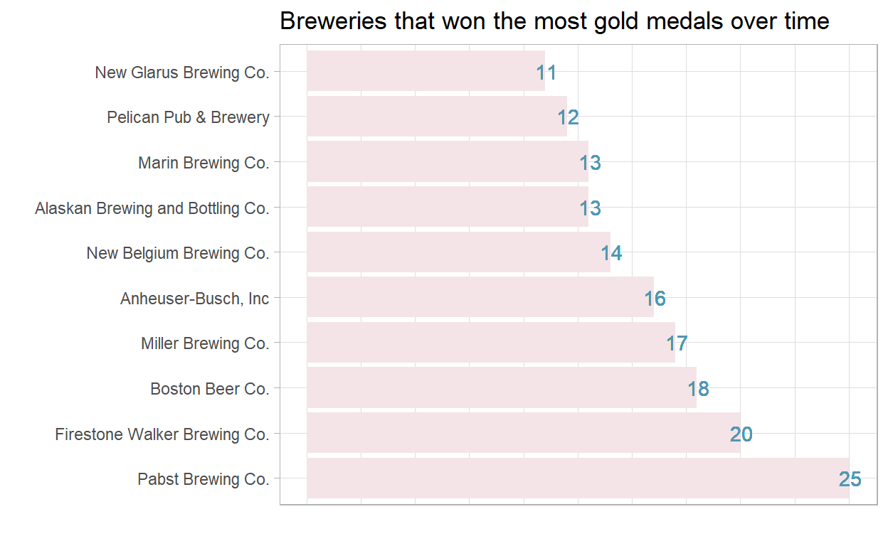
The fct_infreq() orders it from most frequent (which is shown at bottom of plot, because ggplot plots the levels from the bottom going up) to least frequent (shown at top of plot). Visually we see the least frequent at top of the plot, and most frequent at the bottom of the plot.
To see what fct_infreq() does let’s look at the levels.
beer_awards %>%
  filter(medal == "Gold") %>%
  mutate(brewery = fct_lump(brewery, n = 10,
                            ties.method = "first")) %>%
  filter(brewery != "Other") %>%
  mutate(brewery = fct_infreq(brewery)) %>%
  pull(brewery) %>%
  levels()
[1] "Pabst Brewing Co."
[2] "Firestone Walker Brewing Co."
[3] "Boston Beer Co."
[4] "Miller Brewing Co."
[5] "Anheuser-Busch, Inc"
[6] "New Belgium Brewing Co."
[7] "Alaskan Brewing and Bottling Co."
[8] "Marin Brewing Co."
[9] "Pelican Pub & Brewery"
[10] "New Glarus Brewing Co."
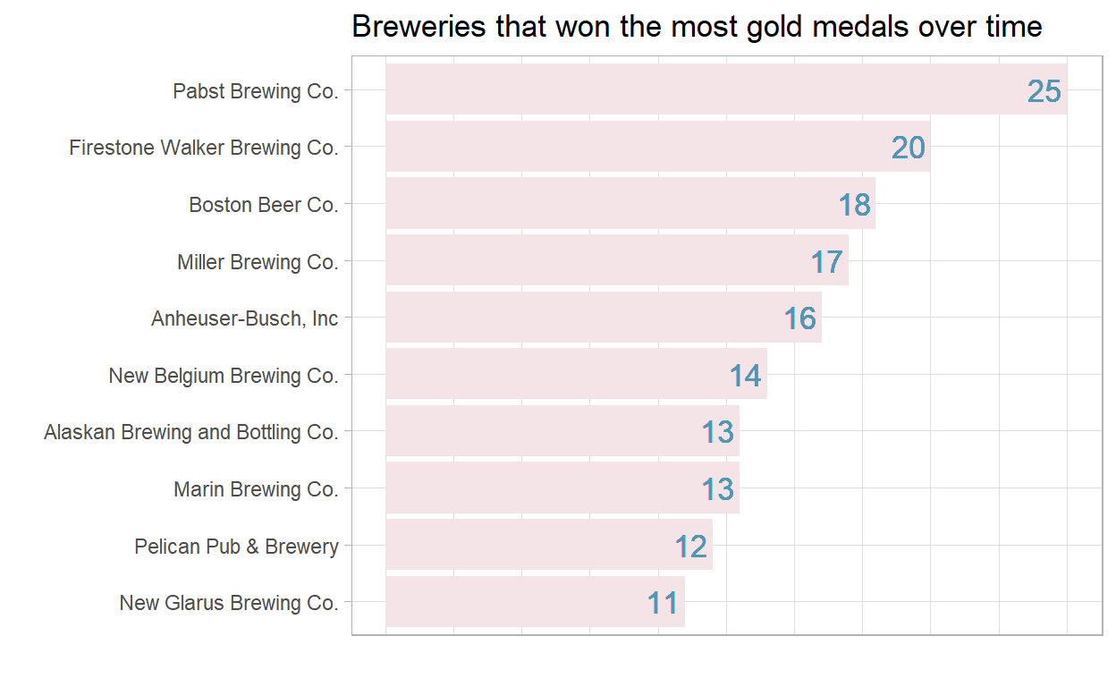
[11] "Other" It is sometimes better to see bar plots in descending order on the visual (i.e. we want to see the most frequent at top of plot, and least frequent at the bottom). This can be accomplished by combining fct_rev() with fct_infreq().
beer_awards %>%
  filter(medal == "Gold") %>%
  mutate(brewery = fct_lump(brewery, n = 10,
                            ties.method = "first")) %>%
  add_count(brewery, medal) %>%
  filter(brewery != "Other") %>%
  # show in decreasing order of winners on plot
  ggplot(aes(y = fct_rev(fct_infreq(brewery)))) +
  geom_bar(fill = "#f4e4e7") +
  geom_text(aes(label = as.character(n),
                x = n + .06), hjust = 1.2,
            colour = "#5196b4",
            size = 4.5,
            position = position_dodge(width = 1)) +
  labs(x = "",
       y = "",
       title = "Breweries that won the most gold medals over time") +
  theme(axis.text.x = element_blank(),
        axis.ticks.x = element_blank())
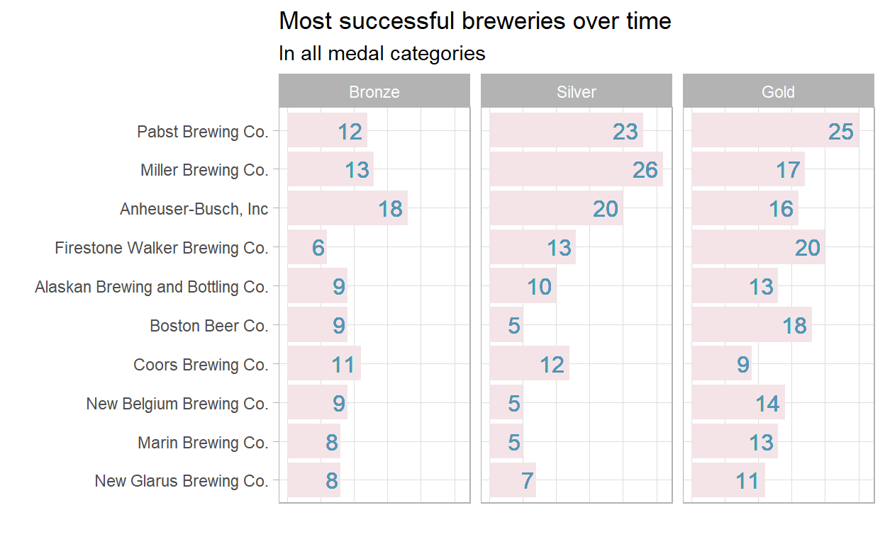
beer_awards %>%
  mutate(brewery = fct_lump(brewery, n = 10)) %>%
  add_count(brewery, medal) %>%
  filter(brewery != "Other") %>%
  ggplot(aes(y = fct_rev(fct_infreq(brewery)))) +
  geom_bar(fill = "#f4e4e7") +
  geom_text(aes(label = as.character(n),
                x = n + .06), hjust = 1.2,
            colour = "#5196b4",
            size = 4.2,
            position = position_dodge(width = 1)) +
  facet_wrap(~ fct_inorder(medal)) +
  labs(x = "",
       y = "",
       title = "Most successful breweries over time",
       subtitle = "In all medal categories") +
  theme(axis.text.x = element_blank(),
        axis.ticks.x = element_blank())
fct_reorder()
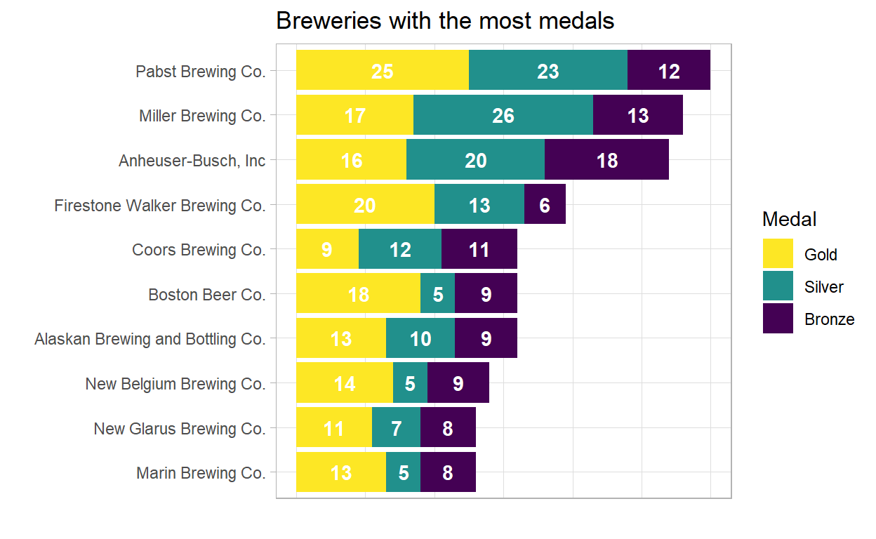
On occasion you may want to reorder to make your visuals easier to read. You can do this using fct_reorder().
fct_reorder(var, some_other_var, some_func) where:
- var: the variable you want to reorder (below this is the
breweryvariable) - some_other_var: what should determine the order that var will be put into? Below we’re going to reorder
breweryby the count of medals the brewery received. - some_func: Is there some summary function that must be applied? For example, should we sum up some_other_var, or take the median of some_other_var for the order of var to be determined by. Below since we have Bronze, Silver and Gold medals we’re going to sum up the counts in each medal category and use that to determine which order
breweryshould be in.
Ultimately we want to plot the most successful breweries from most successful to least successful in the top 10.
beer_awards %>%
  # keep top 10 breweries, lump all the rest into Other
  mutate(brewery = fct_lump(brewery, n = 10)) %>%
  add_count(brewery, medal) %>%
  select(brewery, medal, n) %>%
  distinct() %>%
  # remove the "Other" category because it makes it hard
  # to see all the rest
  filter(brewery != "Other") %>%
  # reorder the brewery by the sum of the number of all
  # medals such that brewery with most medals are at top
  mutate(brewery = fct_reorder(brewery, n, sum)) %>%
  mutate(medal = fct_relevel(medal,
                                "Bronze",
                                "Silver",
                                "Gold")) %>%
  ggplot(aes(n, brewery,
             fill = medal)) +
  geom_col() +
  geom_text(aes(label = n, fontface = "bold"),
            position = position_stack(vjust = 0.5),
            colour = "white") +
  scale_fill_viridis_d() +
  labs(x = "",
       y = "",
       title = "Breweries with the most medals",
       fill = "Medal") +
  theme(axis.text.x = element_blank(),
        axis.ticks.x = element_blank()) +
  guides(fill = guide_legend(reverse = TRUE))
Code
You will find the RMarkdown replica of this post here.
Session Info
Show code
R version 4.1.1 (2021-08-10)
Platform: x86_64-w64-mingw32/x64 (64-bit)
Running under: Windows 10 x64 (build 19043)

Matrix products: default

locale:
[1] LC_COLLATE=English_South Africa.1252
[2] LC_CTYPE=English_South Africa.1252
[3] LC_MONETARY=English_South Africa.1252
[4] LC_NUMERIC=C
[5] LC_TIME=English_South Africa.1252

attached base packages:
[1] stats     graphics  grDevices utils     datasets  methods
[7] base

other attached packages:
 [1] forcats_0.5.1   stringr_1.4.0   dplyr_1.0.7     purrr_0.3.4
 [5] readr_2.0.1     tidyr_1.1.3     tibble_3.1.5    ggplot2_3.3.5
 [9] tidyverse_1.3.1 formatR_1.11

loaded via a namespace (and not attached):
 [1] httr_1.4.2        sass_0.4.0        viridisLite_0.4.0
 [4] bit64_4.0.5       vroom_1.5.5       jsonlite_1.7.2
 [7] modelr_0.1.8      bslib_0.3.0       assertthat_0.2.1
[10] highr_0.9         cellranger_1.1.0  yaml_2.2.1
[13] pillar_1.6.4      backports_1.2.1   glue_1.4.2
[16] digest_0.6.28     rvest_1.0.2       colorspace_2.0-2
[19] htmltools_0.5.2   pkgconfig_2.0.3   broom_0.7.9
[22] haven_2.4.3       scales_1.1.1      distill_1.3
[25] tzdb_0.1.2        downlit_0.2.1     generics_0.1.1
[28] farver_2.1.0      ellipsis_0.3.2    DT_0.19
[31] withr_2.4.2       cli_3.0.1         magrittr_2.0.1
[34] crayon_1.4.2      readxl_1.3.1      evaluate_0.14
[37] fs_1.5.0          fansi_0.5.0       xml2_1.3.2
[40] tools_4.1.1       hms_1.1.0         lifecycle_1.0.1
[43] emoji_0.2.0       munsell_0.5.0     reprex_2.0.1
[46] compiler_4.1.1    jquerylib_0.1.4   rlang_0.4.12
[49] grid_4.1.1        rstudioapi_0.13   htmlwidgets_1.5.4
[52] crosstalk_1.1.1   labeling_0.4.2    rmarkdown_2.11
[55] gtable_0.3.0      codetools_0.2-18  DBI_1.1.1
[58] curl_4.3.2        R6_2.5.1          lubridate_1.7.10
[61] knitr_1.36        fastmap_1.1.0     bit_4.0.4
[64] utf8_1.2.2        stringi_1.7.5     parallel_4.1.1
[67] Rcpp_1.0.7        vctrs_0.3.8       dbplyr_2.1.1
[70] tidyselect_1.1.1  xfun_0.27
Further Resources
- Chapter on Factors in
R for Data Science. - {forcats} Tidyverse Page.
- Vignette on {forcats} by Emily Robinson.
- David Robinson’s TidyTuesday screencasts often include much factor wrangling.